The Sun, quite obviously, is the primary driving force behind weather and climate here on planet Earth. Solar insolation changes with latitude due to the curvature of the Earth, and with season due to the 23° tilt of the Earth’s rotation axis relative to the plane of its orbit about the Sun. Changes in the Earth’s orbit and axial tilt are now recognized as key factors in the long term changes to Earth’s climate that produce ice ages and warm periods. However, we now know that the radiative output of the Sun changes with time. This raises the important question of how much solar variability might influence climate change.
In the 1920s Milutin Milanković suggested that changes in the Earth’s orbit and axial tilt were connected to changes in its climate. These changes are now widely recognized as natural drivers of climate change. The fact that the Earth’s orbit about the Sun is slightly elliptical provides one source of variation (1). The Earth is currently about 3.5% closer to the Sun in early January than it is in early July. This makes northern winters somewhat milder and southern winters somewhat more severe. However, this isn’t the way it has always been. This eccentricity of the Earths orbit changes over time scales of about 100,000 years due to the gravitational attraction of other planets. The timing of the Earth’s closest approach to the Sun shifts through the seasons as the Earth’s rotation axis precesses with a period of about 26,000 years (2) (The Earth’s north pole current points at the star Polaris but will point at Vega in another 12,000 years.). The actual tilt of the Earth’s rotation axis to the plane of its orbit about the Sun also changes – over time scales of about 41,000 years (3). These three changes in the physical relationship between the Earth and the Sun are solidly linked to changes in Earth’s climate.
Other naturally occurring sources of climate change include volcanic eruptions and meteor impacts. These have the nearly immediate effect of cooling as high altitude particulates block sunlight from reaching the Earth’s surface. Climate is also influenced by its own internal variations – the El Niño-Southern Oscillation and the North Atlantic Oscillation. Solar variability, as evidenced by sunspots and, as we will see, by radioisotopes in tree rings and in ice cores, is also identified as a natural source of climate change. In this essay we will focus on the connections between solar variability and climate. But first, we must understand more about sunspots, solar variability, and the Sun’s magnetic activity.
Sunspots and Solar Variability
Sunspots, dark spots that appear on the Sun’s surface and last for anywhere from hours to months, were first noted in western cultures after the invention of the telescope in the early 1600s. However, the existence of sunspots was well known many centuries earlier by Chinese and other eastern observers (Some sunspot groups are large enough to be seen without the aid of a telescope when the Sun can be viewed at through smoke or fog).
The invention of the telescope allowed for daily observations of sunspots. This led to the early discovery of the rotation of the Sun – a 27-day rotation period on average but faster near the equator than at higher latitudes (the Sun is a ball of ionized gas and does not rotate rigidly). Surprisingly, astronomers were observing sunspots and making drawings of their shape and positions for well over 200 years before the 11-year sunspot cycle was discovered. In 1843 Heinrich Schwabe, a German amateur astronomer, reported on his observations of what we now refer to as the sunspot cycle – a cycle of about 11-years length in which the number of sunspots seen on the Sun waxes and wanes. Schwabe’s observations from 1826 to 1843 clearly showed two of these cycles.
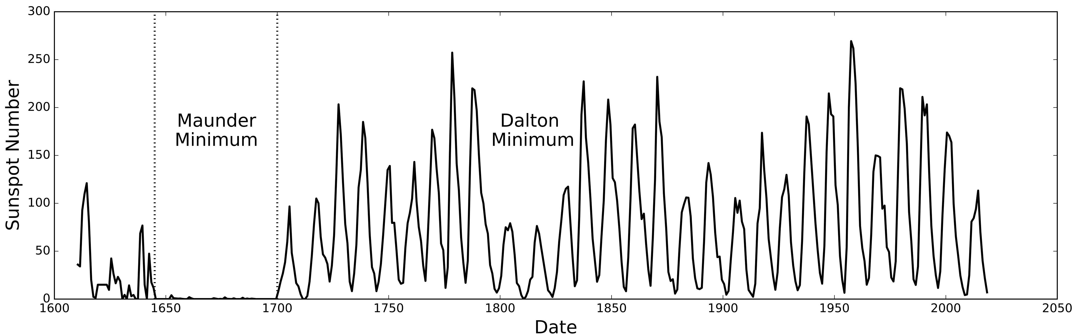
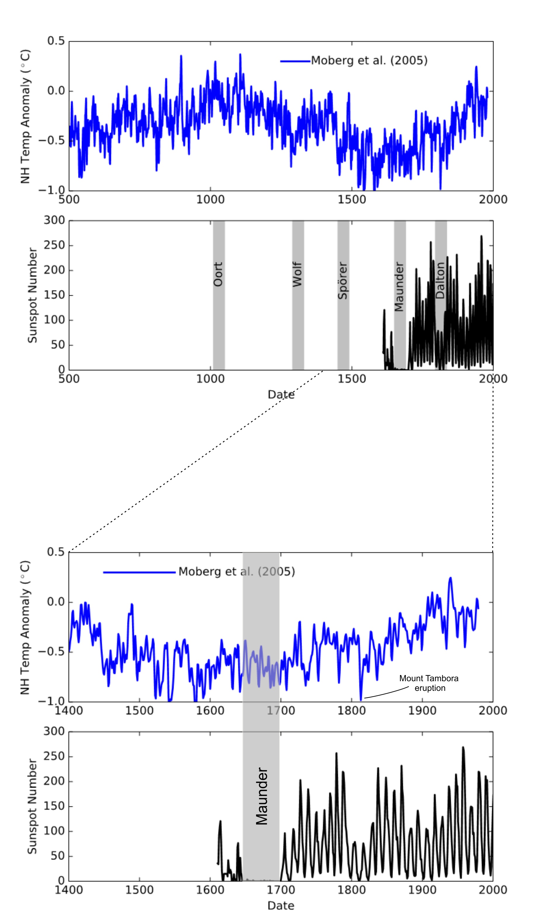
Shortly after Schwabe published his results, Rudolf Wolf (an astronomer at the Bern Observatory and later at the Zurich Observatory) instituted a daily observing program to track the sunspot cycle and extended his catalog of observations backward in time using observation by earlier observers. Wolf recognized that it was difficult to see and count small sunspots but far easier to count sunspot groups. (Even the earliest observers had noticed that sunspot appear in clusters or groups.) This led Wolf to define a sunspot number as ten times the number of groups plus the number of individual spots – a definition we still use today albeit with slight variations (a recent revision is referred to as Version 2.0). The 400+ year record of yearly averages of the daily sunspot numbers is shown in Figure 2. While the sunspot number drops to near zero at the minimum of each 11-year sunspot cycle, this record also shows an example of a Grand Minimum – the Maunder Minimum – a period of decades (that should have included several sunspot cycles) with virtually no sunspots at all.
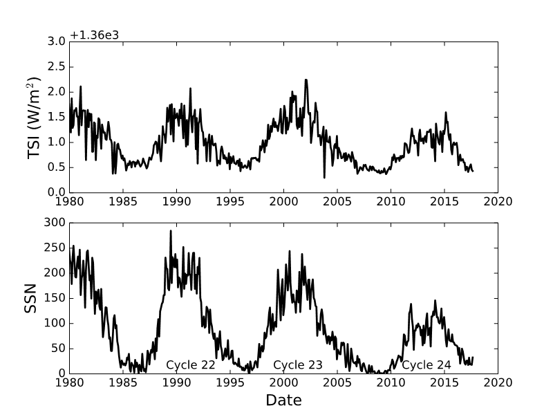
One would think that the presence of dark sunspots would make the Sun darker at sunspot cycle maxima and brighter at sunspot cycle minima. Space age observations show the opposite! Measurements of the Sun’s irradiance have been made from a series of spacecraft above the Earth’s atmosphere since the late 1970s. These measurements of the so-called solar constant (about 1360 Watts per square meter) do show dips associated with the passage of sunspot groups, but they also show an overall increase in irradiance as the sunspot numbers increase. This variation in the Total Solar Irradiance (TSI) is shown in Figure 3 using data (Version 42_65_1709) compiled by Claus Fröhlich at the Physikalisch-Meteorologisches Observatorium Davos/World Radiation Center (PMOD/WRC) in Davos, Switzerland.
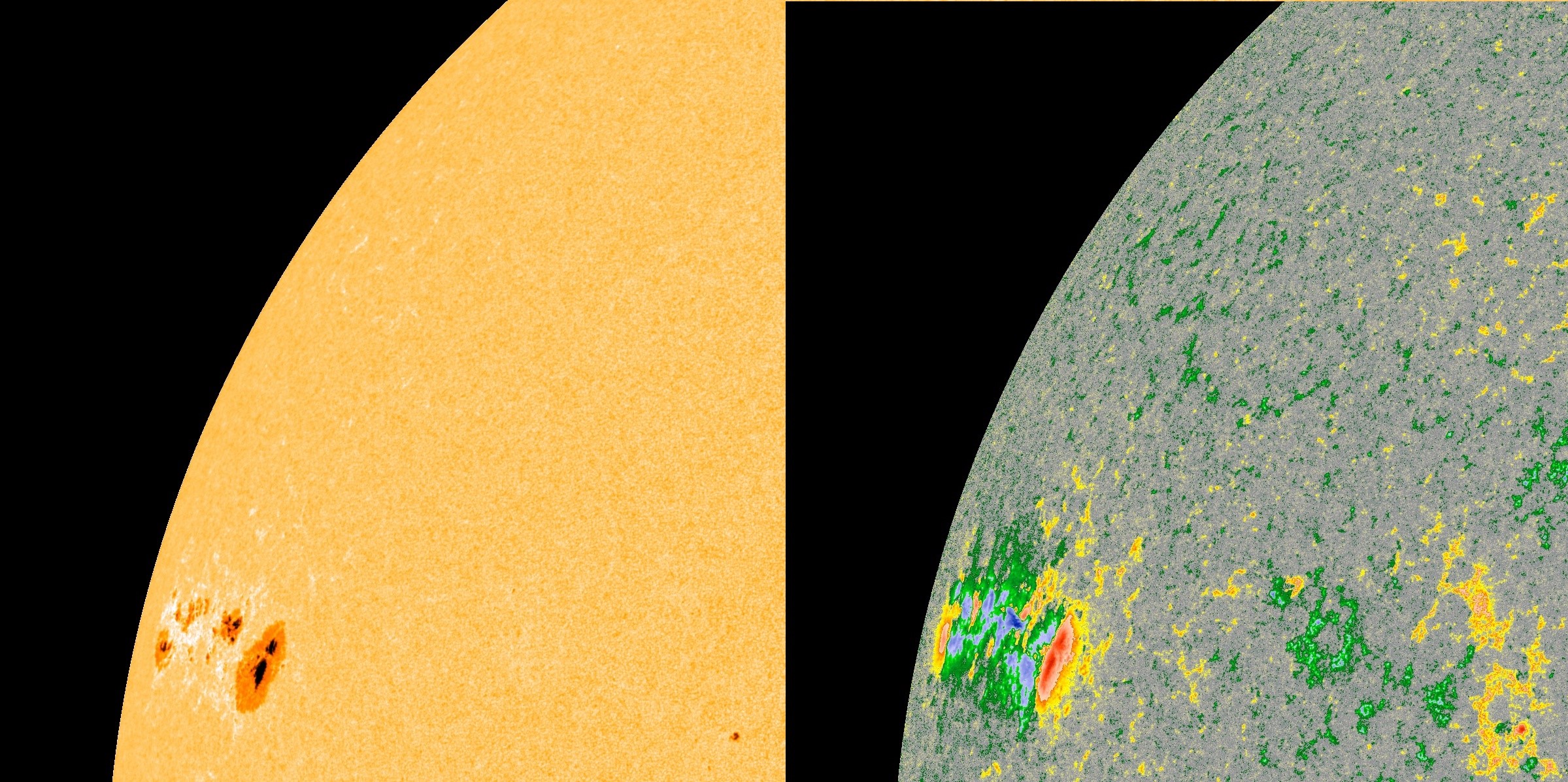
This puzzling result, with the Sun being brighter when there are more sunspots, is explained by the true nature of sunspots and the sunspot cycle. Over 100 years ago George Ellery Hale, founder and director of the Mount Wilson Observatory in Pasadena, California, discovered that sunspots are regions where very intense magnetic fields loop up out of and back into the Sun. These magnetic fields are intense enough to nearly choke off the flow of heat from the Sun’s interior. The boiling motions of the ionized gases cannot push aside the magnetic field in sunspots to reach the surface. This makes sunspots darker and cooler than other regions on the Sun’s surface (sunspots have a temperature of about 3,800 degrees Kelvin, which contrasts with the surrounding solar surface at roughly 5,800 degrees Kelvin). Further investigation shows that the entire surface of the Sun is populated with smaller, weaker magnetic features called faculae that appear bright, particularly when seen near the edge or limb of the Sun. This is illustrated in Figure 4 using images from the Helioseismic and Magnetic Imager (HMI) on the NASA Solar Dynamics Observatory (SDO) satellite. While the bright faculae can be seen anywhere on the Sun, they are far more frequent and brighter around sunspot groups (also referred to as active regions). Thus, as the number of sunspots increases so do the number of faculae, this makes the Sun brighter at sunspot cycle maxima.
Magnetic Fields and the Solar Cycle
We can measure magnetic fields on the Sun because of the Zeeman effect. In the presence of magnetic fields the structures of atoms and ions are changed. Electrons orbiting in one direction will have more energy than electrons in the same orbit traveling in the opposite direction. This splits energy levels and causes the light that is emitted or absorbed to be polarized. Both the strength and the direction of magnetic fields in the Sun’s atmosphere can be determined using a spectrograph with polarizing filters. Solar magnetic fields have been measured this way since the pioneering work of George Ellery Hale in 1908. These measurements show that the sunspot cycle is just one part of a more involved magnetic cycle that takes about 22 years to complete.
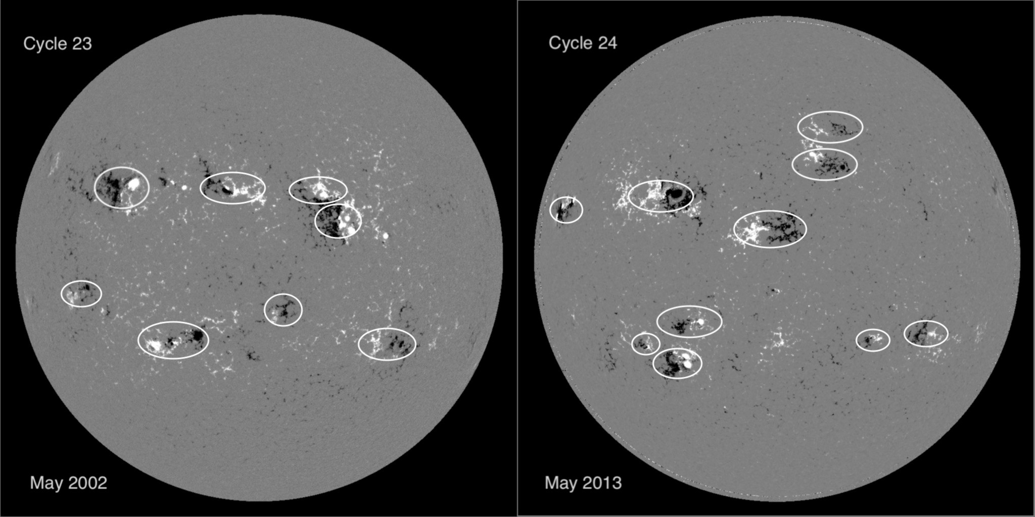
Figure 5 shows a pair of magnetic images (magnetograms) of the Sun taken 11 years apart. This figure illustrates several key characteristics of the Sun’s magnetic cycle:
- Sunspot groups tend to be spread out in an east-west direction with spots on the right being of one polarity (e.g. positive or outward pointing) while spots on the left are of the opposite polarity.
- Sunspot groups in one hemisphere have right-positive and left-negative while groups in the other hemisphere have the opposite – right-negative and left-positive.
- This configuration of hemispheric active region polarity reverses during the next 11-year sunspot cycle as seen in the right hand image in Figure 5.
These properties are known collectively as Hale’s Law and are key to understanding how the solar cycle works.
The Sun’s 22-year magnetic cycle is illustrated in Video 1 below. Maps of the magnetic field across the full surface of the Sun are constructed by "peeling off" the magnetic field data from near the central meridian as the Sun rotates over the course of about 27 days. (Here positive fields are yellow and negative fields are blue). This series of maps, compiled over the course of thirty years, illustrates how active regions emerge in two bands – one on either side of the equator. The individual active regions drift to the right as they are carried along by the Sun’s differential rotation (24 days near the equator). Over the course of each cycle the active latitude bands drift toward the equator and then die out as new bands (with opposite magnetic polarities as given by Hale’s Law) emerge at higher latitudes to start the process again. At higher latitudes we see the remains of the active region magnetic fields drift to the left in the slower rotational flow (36 days near the poles) and drift toward the poles in what is referred to as the meridional flow.
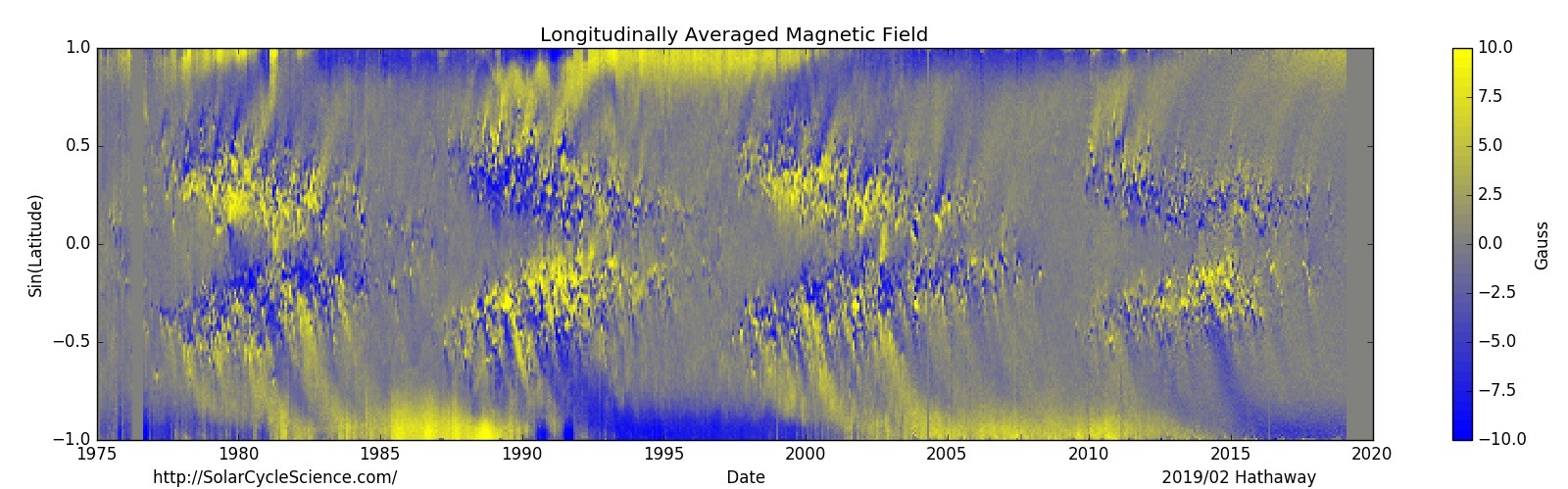
Figure 6 shows, in what is naturally referred to as a butterfly diagram, a synopsis of the data shown in Video 1. The longitudinal average of the magnetic field in each 27-day magnetic map is plotted as a function of latitude. The time history shows the 22-year magnetic cycle along with two more (beyond Hale’s Law) key characteristics of the Sun’s activity cycle.
(1) The first of these characteristics is referred to as Joy’s Law – active regions have a characteristic tilt away from a purely east-west orientation. This tilt places the preceding (in the direction of rotation or to the right) parts of active regions closer to the equator than the following (opposite magnetic polarity) parts. A result of Joy’s Law is a preponderance of following polarity magnetic field on the poleward sides of the "butterfly wings" and of preceding polarity on the equatorward sides. With Hale’s Law this gives butterfly wings with the opposite configuration in the opposing hemisphere and in the adjacent cycles.
(2) The second of these characteristics is the polar field reversals, which occur near the time of sunspot cycle maximum for each cycle. These reversals are caused by the latitudinal transport of the active region magnetic fields in the poleward meridional flow that was revealed in Video 1. Since, due to the Hale and Joy polarity laws, the higher reaches of the active latitudes are dominated by following polarity magnetic fields, this magnetic polarity is carried off to the poles where it weakens and then reverses the polar fields in each hemisphere.
These characteristics of the Sun’s magnetic cycle provide us with a model for how the sunspot cycle arises – a magnetic dynamo model. Although details are still debated within the scientific community, a simplified model based on the works of Horace Babcock (at the Mount Wilson and Palomar Observatories) and Robert Leighton (at the California Institute of Technology) in the 1960s stands the test of time. This four-stage process is illustrated in Figure 7.
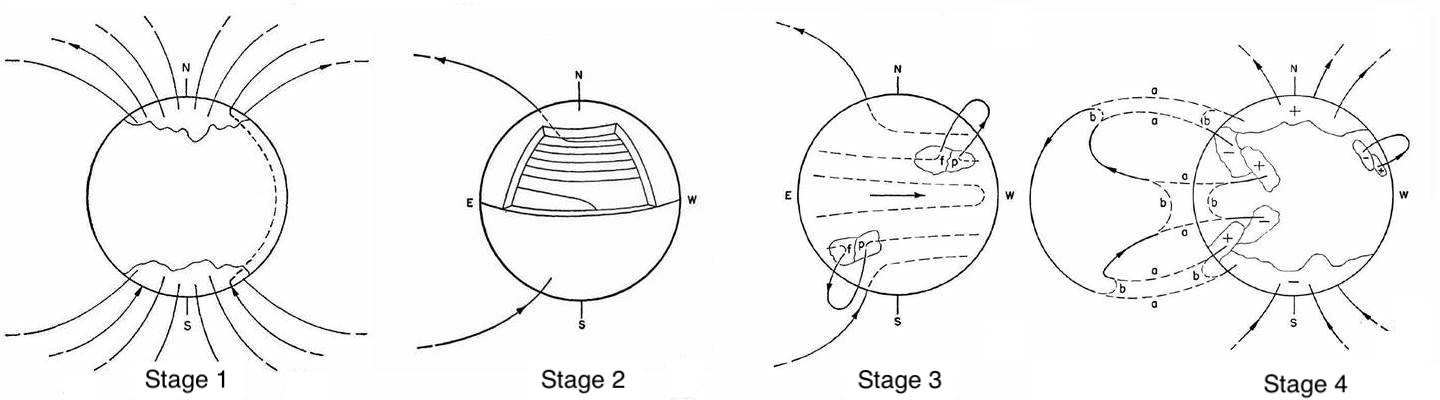
Stage 1 is near sunspot cycle minimum with the Sun’s magnetic field dominated by the polar fields, each of opposite polarity. This field threads north-south through the Sun’s interior to link the two polarities together. In stage 2, this internal magnetic field is stretched out in the east-west direction and amplified by the Sun’s differential rotation. In stage 3 this largely east-west field (but with a slight north-south tilt giving Joy’s Law) becomes strong enough to become buoyant and loops rise through the surface to form active regions with sunspots. This process naturally produces both Hale’s Law and (to some extent) Joy’s Law with the preceding polarity matching the polar field polarity at minimum and the following polarity (at a higher latitude) opposite to the initial polar fields. In stage 4 the process is completed by the poleward transport of the following polarity magnetic field to reverse the polarity of the polar fields. At lower latitudes, the leading polarity has been replaced by following polarity as the active latitudes move equatorward and eventually the opposite leading polarities on either side of the equator cancel each other out. The four stages then repeat with opposite polarities to complete the 22-year magnetic cycle.
An important aspect of this process – born out by observations – is that the strength of the Sun’s polar fields at the time of cycle minimum predicts the size of the following cycle. These polar fields and their interior connections are the seed fields for the next cycle.
Magnetic Fields and Solar Activity
Solar magnetic fields do far more than simply produce sunspots, active regions, and faculae. The magnetic field in active regions can become stressed by fluid motions below the surface and by the emergence of additional magnetic flux. Stressed magnetic fields can erupt explosively to produce a range of solar activity – solar flares (explosions the size of the Earth with the energy equivalent of a million atomic bombs) and coronal mass ejections (a billion tons of matter blown off of the Sun at speeds in excess of several million kph). During cycle maxima there can be several of these each day. On the other hand, at cycle minima days can go by without any of these eruptive events.
Magnetic fields are also critical to the process of heating the Sun’s corona and driving the solar wind. These magnetic processes are illustrated in Video 2 – derived from images of the corona obtained with the Large Angle and Spectrometric Coronograph (LASCO) on the ESA/NASA Solar and Heliospheric Observatory (SOHO) Mission. Video 2 shows the flow of the solar wind streaming off of the Sun over the course of a month being interrupted by coronal mass ejections.
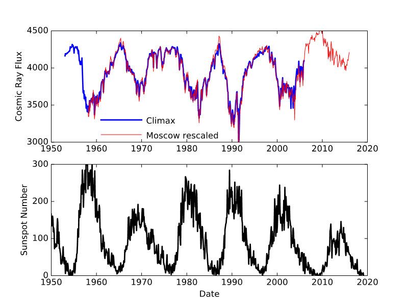
The structure of the solar wind, and the frequency of coronal mass ejections, changes with the solar cycle. The solar wind and the magnetic field threading through it are far more tangled and complicated at solar cycle maxima. This leads to more frequent auroral displays at cycle maxima. It also has other consequences – the influx of cosmic rays to Earth is diminished when the Sun is active and is enhanced when the Sun is inactive. This is shown in Figure 8 with monthly averaged cosmic ray fluxes from two stations – Climax, Colorado, USA and Moscow, Russia.
This variation in the cosmic ray radiation levels at Earth changes the production of radioisotopes in the Earth’s upper atmosphere. Cosmic rays are comprised of elementary particles – electrons, protons, alpha particles and the nuclei of even heavier elements – moving with such speed and such energy that they cause nuclear reactions when they hit atoms and molecules in Earth’s atmosphere. These nuclear reactions produce the radioactive isotopes 14C and 10Be. The 14C gets incorporated into plants while the 10Be precipitates and get incorporated in ice. The level of solar activity thousands of years in the past can be estimated by measuring the variation in the abundance of 14C in tree rings and 10Be in ice cores. This process is not without its problems. While solar cycle related changes in the solar wind influence the flux of cosmic rays, this flux is also influenced by the Earth’s magnetic field and its variation with latitude and time.
A key result of the studies of solar variability based on radioisotopes is the discovery that the Maunder Minimum is just one of many Grand Minima. Other named Grand Minima include the Spörer Minimum (~1470 AD), the Wolf Minimum (~1310 AD), and the Oort Minimum (~1030 AD). Estimates are that there have been about 30 Grand Minima over the last 8000 years. Another key result is the discovery that Sun’s magnetic cycle extended through the Maunder Minimum, albeit at a reduced level that did not produce sunspots. This suggests that the Sun’s magnetic cycle continues, even when sunspots are not produced. In fact we do see the emergence of many weaker magnetic features at the Sun’s surface that do not produce sunspots but contribute to the magnetic cycle. It has become clear that the emerging magnetic field must be stronger than some critical level to produce sunspots.
Solar Activity and Climate
Connections have long been made between solar activity and climate. The connection most often cited is between the Maunder Minimum and the Little Ice Age. This has led some to conclude that the decrease in solar activity over the last few cycles will lead to a Grand Minimum and another little ice age. The evidence indicates that this is highly unlikely on two counts:
(1) Predictions for the size of the next cycle, Cycle 25, do not indicate that it will be the start of a Grand Minimum. Most indicators (e.g. the current strength of the Sun’s polar magnetic field) are for a cycle similar in strength to the current cycle (Cycle 24, which is presently declining and expected to reach its minimum end of 2019 or in 2020).
(2) Even if the Sun did drop into a Grand Minimum, any cooling would be overpowered by global warming due to anthropogenic causes.
Many studies have been (and continue to be) published on global temperature changes. Some are based on instrumental temperature measurements. Others, extending back further in time, are based on proxies for temperature. These proxies include tree rings (annual ring width, density, radioisotopes), ice cores (accumulation width, melt layers, radioisotopes), and bore holes (temperature as a function of depth).
One reconstruction based on proxies produced by Anders Moberg and his colleagues extends back 2000 years and is shown in Figure 9 . Key characteristics of this temperature record include a medieval warm period around 1000 AD and a cool period (the Little Ice Age) around 1600. While this cool period does extend into the time of the Maunder Minimum, it started much earlier and was more severe in the 1500s. The dramatic dip in temperature in the Dalton Minimum is 1816, the "year without a summer". This event is firmly attributed to the cooling effects of the volcanic eruption of Mount Tambora in April 1815.
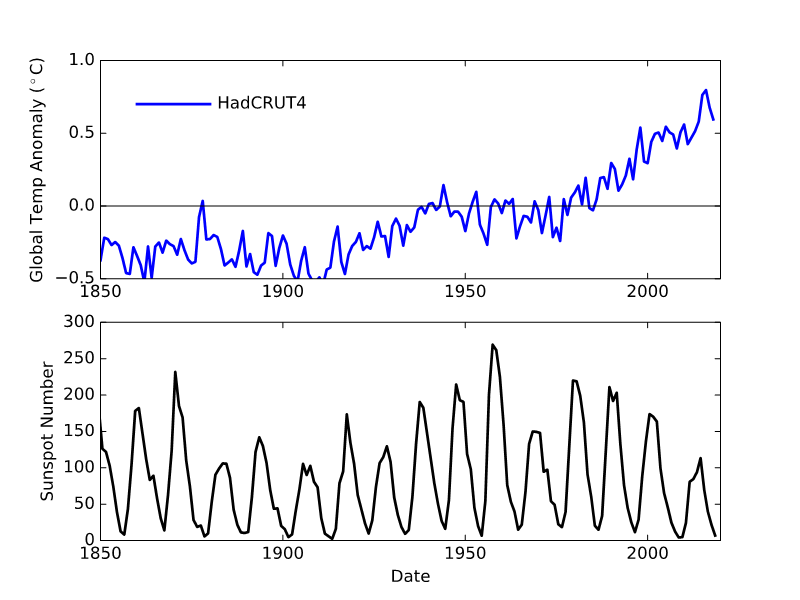
The dataset from the Climatic Research Unit (University of East Anglia) in conjunction with the Hadley Centre (UK Met Office) – HadCRUT4 – extends the instrumentally measured temperature record from the present back to 1850. In Figure 10, the yearly average global temperature anomaly (relative to 1961-1990) is plotted along with the yearly average sunspot number V2.0. The first 100 years of the global temperature record seems to mimic the sunspot numbers with lower temperatures associated with the smaller cycles at the start of the 1900s and higher temperatures associated with the larger cycles in the mid-1900s. However, the rapid rise in temperature since the mid-1900s runs counter to the concurrent drop in sunspot cycle amplitudes.
Years ago, prior to the Version 2.0 reconstruction of the sunspot record, there seemed to be a strong correlation between sunspot numbers and global temperature – primarily due to an apparent increase in cycle amplitude since the Maunder Minimum. The correlation was stronger than what could be attributed to the 0.1% change in solar irradiance. This led to a search for other solar cycle related factors that might influence climate. Two factors stood out – changes in the Earth’s upper atmosphere due to solar cycle changes in ultraviolet emissions and changes in cloudiness due to increased cosmic ray fluxes. Research into both factors never gave conclusive answers. With Version 2.0 the correlation between sunspot numbers and global temperatures is much weaker.
When all factors are accounted for (volcanoes, El Niño, greenhouses gases, etc.) it now appears that the impact of solar activity on climate is simply the impact due to the 0.1% change in solar irradiance associated with sunspots and faculae. When this variation is entered into global climate models it translates to a 0.1 °C change in global temperature. This is commensurate with the temperatures seen during the Maunder and Dalton minima. It indicates that even if the Sun does enter another Grand Minimum (which is unlikely for the next cycle), it will not produce another little ice age.
References and Data Sources
- Moberg A, Sonechkin DM, Holmgren K, Datsenko NM, and Karlén W (2005) Highly variable Northern Hemisphere temperatures reconstructed from low- and high-resolution proxy data. Nature 433: 613–617
- Babcock HW (1961) The Topology of the Sun's Magnetic Field and the 22-Year Cycle. The Astrophysical Journal 133: 572-587
- Sunspot Index and Long-term Solar Observations
- The ESA/NASA Solar and Heliospheric Observatory (SOHO)
- The NASA Solar Dynamics Observatory (SDO)
- Physikalisch-Meteorologisches Observatorium Davos / World Radiation Center (PMOD/WRC): Total Solar Irradiance (TSI)
- Hadley Climate Research Unit temperature (HadCRUT4)
- Dataset from Moberg A et al., 2005, Nature 433: 613-617: 2,000-Year Northern Hemisphere Temperature Reconstruction. World Data Center for Paleoclimatology, Boulder, and NOAA Paleoclimatology Program
Want to Know More?
- Usoskin IG (2017) A history of solar activity over millennia Living Rev. Sol. Phys. 14: 3; doi: 10.1007/s41116-017-0006-9
- Hathaway DH (2015) The Solar Cycle Living Rev. Sol. Phys. 12: 4; doi: 10.1007/lrsp-2015-4
- Haigh JD (2007) The Sun and the Earth’s Climate Living Rev. Sol. Phys. (2007) 4: 2; doi: 10.12942/lrsp-2007-2
- U.S. Global Change Research Program (USGCRP) (2018) Fourth National Climate Assessment
Other Articles by This Author
Further Articles in  Planetary Science
 This work is distributed under a Creative Commons Attribution ShareAlike 4.0 International License (CC BY-SA 4.0). Its use, distribution and reproduction in other forums is permitted provided both the original author(s) and Capeia are accredited, and the license is unchanged (CC BY-SA 4.0). Images or other third party material in this article are covered under the article’s Creative Commons license unless otherwise indicated; if the material is not covered under a Creative Commons license, users will need to obtain permission from the license holder before it can be reproduced.
Responses